STM32 Guitar Tuner
February 13, 2020
Table of contents
Introduction
I built a guitar tuner using an electret microphone, an ARM Cortex-M3 processor, and a 128x32 OLED display. For those unfamiliar with this style of guitar tuner, it operates as follows: the user plays a guitar string that they are trying to tune, and the OLED displays tuning instructions (tune up, tune down, or in tune).
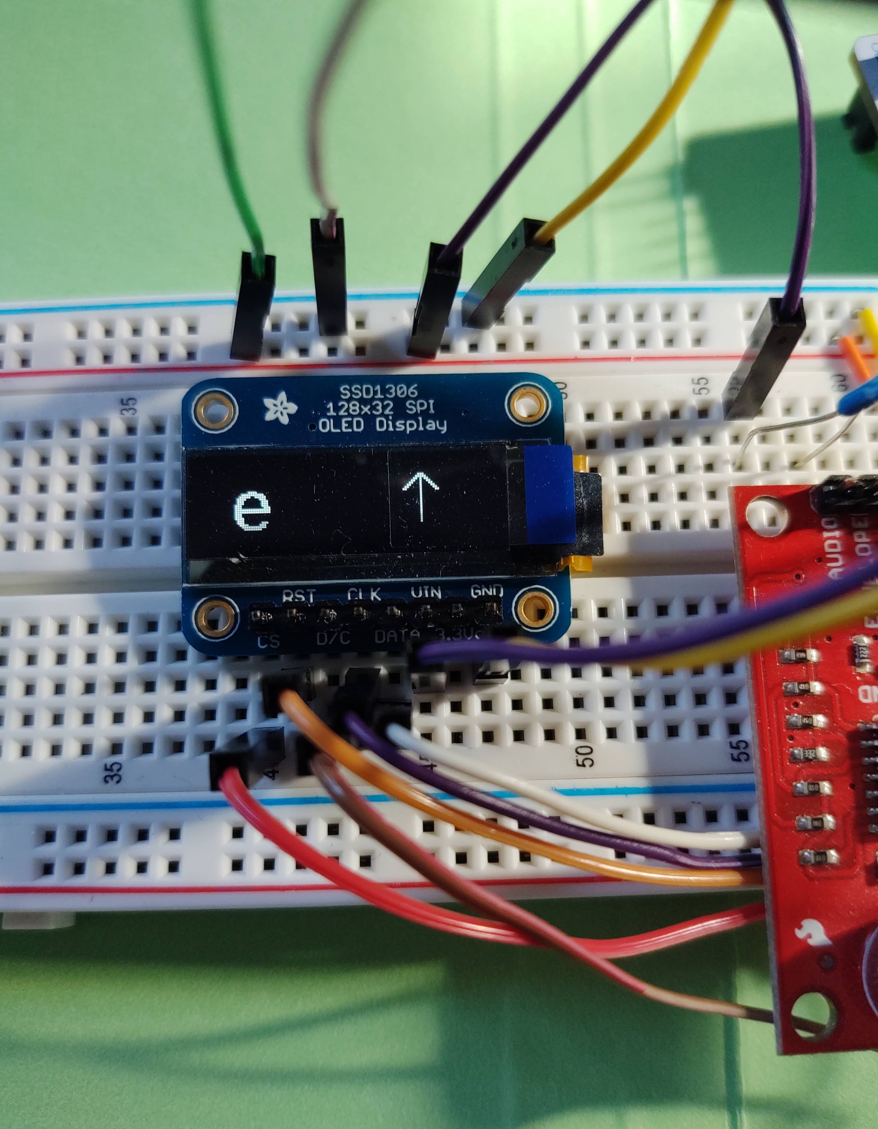
Parts used
- NUCLEO-STM32F103RB Development board
- SSD1306 OLED Display (128 x 32)
- SparkFun Sound Detector
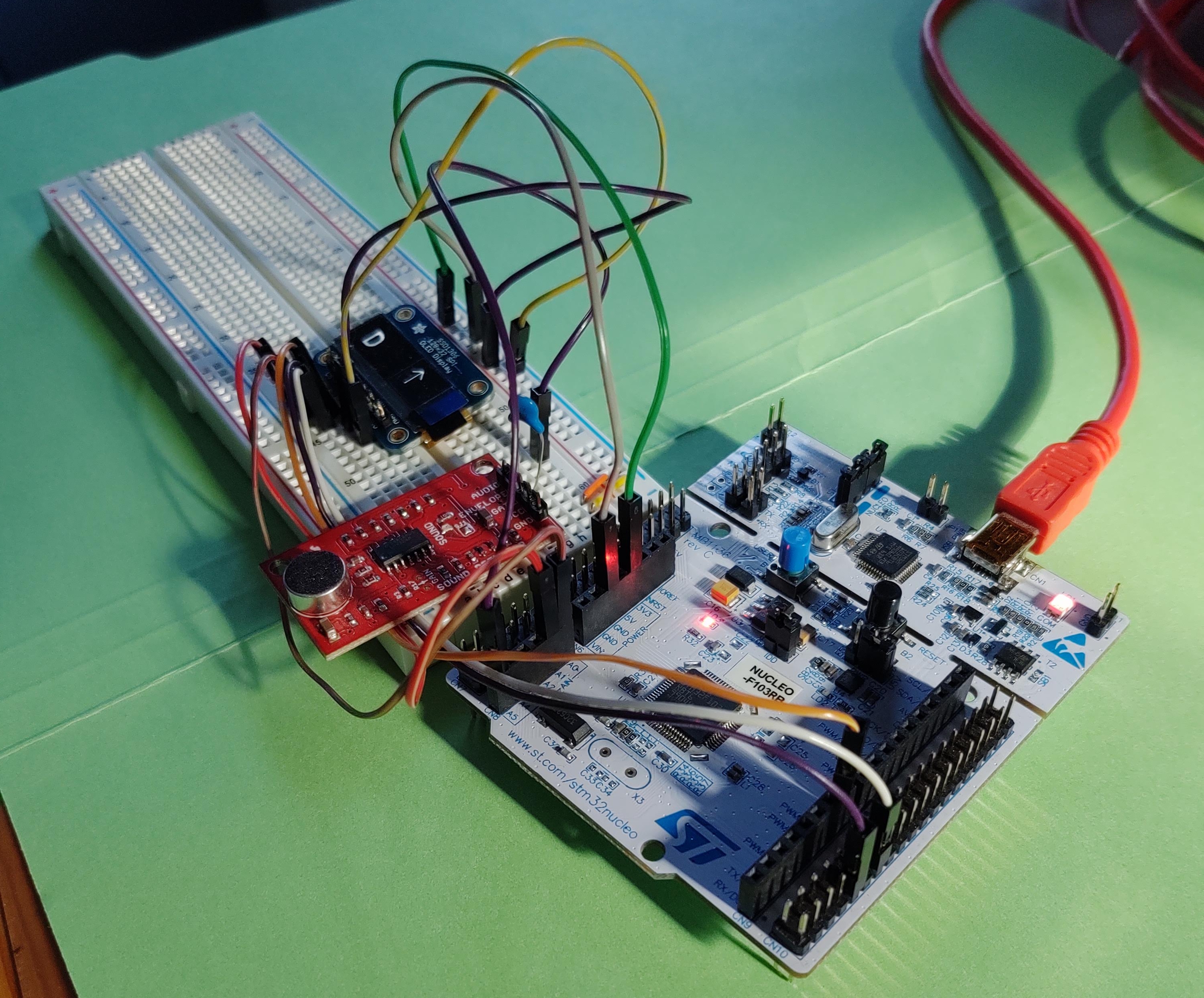
Approach/Analysis
Going into this project I had minimal experience programming the STM32F103 board and working with discrete signals. I was not sure how I would detect fundamental frequency from a time domain recording of a guitar string.
I started this project by taking samples from the ADC on the STM32 and sending them over UART to my laptop so I could analyze the signals using Python. Since the highest frequency guitar string is the e string at 330Hz, I had to sample at a frequency of at least 660Hz. I gave myself some cushion and chose to use a 1KHz sampling rate. This also made the timer interrupt setup simple.
The below Python notebook describes how I came up with a way to detect fundamental frequency of a recorded guitar string.
In standard guitar tuning the six notes and their ideal frequencies are as follows:
| Note | Frequency (Hz) |
|---|---|
| E | 82 |
| A | 110 |
| D | 147 |
| G | 196 |
| B | 247 |
| e | 330 |
from helper import *
import numpy as np
import os

WAVEFORM_DIR = 'pickled_waveforms/raw_waveforms'
FFT_DIR = 'pickled_waveforms/frequency_domain_waveforms'
SIGNAL_LENGTH = 256

strings = ['E', 'A', 'D', 'G', 'B', 'e']
%matplotlib inline
plt.rcParams["figure.figsize"] = (20,30)
Import signals captured by the ADC on the STM32. Signals were captured and pickled to easily access at later times.
raw_signals contains 24 signals of 256 float values captured from the microphone sampled at 1KHz by the ADC. Four samples were captured for all 6 guitar strings, hence 4*6=24 samples.
fft_signals also contains 24 signals, with 4 signals for all 6 strings. These signals are frequency domain signals obtained by performing a FFT on the STM32, with DC component and 60Hz components set to 0.
raw_signals = dict()
fft_signals = dict()
for each in strings:
    raw_signals[each] = read_pickle_file(os.path.join(WAVEFORM_DIR, ‘guitar%s_256_4.txt’%each))
    fft_signals[each] = read_pickle_file(os.path.join(FFT_DIR, ‘fft_%s_256_4.txt’%each))

# freq = np.fft.fftfreq(SIGNAL_LENGTH, 0.001)
Let’s take a look at the frequency domain signals for each guitar string. The ideal fundamental frequency of each guitar string is plotted in red.
fig, a = plt.subplots(6,4)
for row, st in enumerate(fft_signals.keys()):
    for i in range(4):
        freq = fft_signals[st][i].keys()
        mag = fft_signals[st][i].values()
        a[row][i].stem(freq, mag, use_line_collection=True)
        a[row][i].stem([string_freq[st]], [max(mag)], 'r:', use_line_collection=True)
        a[row][i].set_title(st)
        a[row][i].grid(which='both')
        a[row][i].minorticks_on()
plt.show()
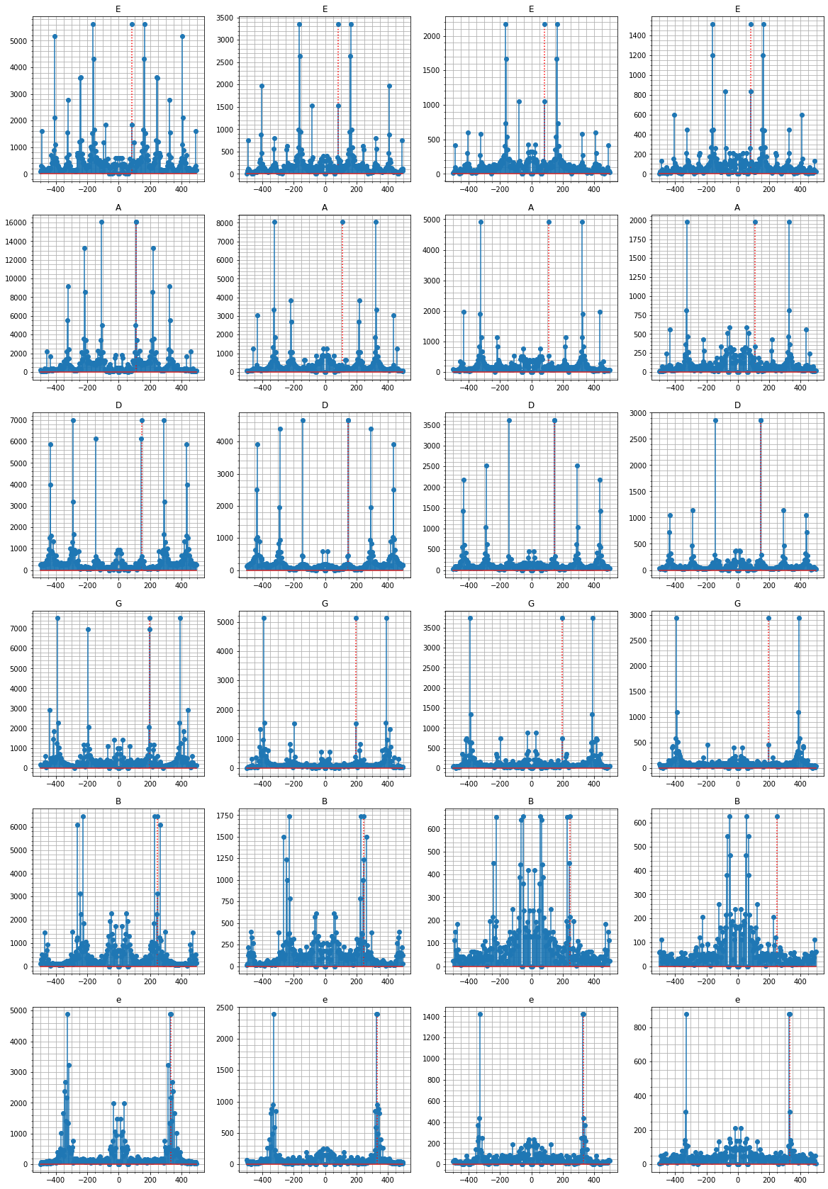
As can be seen, the ideal frequency does not always match the greatest frequency component of the frequency domain signals. Each guitar string seems to have a unique ‘footprint’. For the lower frequency strings, we see a lot of spikes in the frequency domain signal due to harmonics. Predicting a signals fundamental frequency will prove difficult, since harmonics can be much greater in magnitude than the fundamental frequency for a given string.
Take a look at the A string samples. In the second, third, and fourth samples, the fundamental frequency (110Hz) is dwarfed by it’s harmonics. The third harmonic of A (330Hz) is also the fundamental frequency of the high e string. Similarly, the third harmonic of E (247Hz) is also the fundamental frequency of the B string.
At this point I realized that predicting the fundamental frequency of a guitar string recording will take two steps:
- Predict the guitar string being played
- Estimate the fundamental frequency by taking a weighted average of FFT coefficients around that guitar string
Predicting the guitar string from frequency domain signal
To predict the guitar string being played, I had to find a way to classify frequency domain signals. I already had 4 samples of each guitar string in the frequency domain so I used this information to develop an algorithm to classify new signals. I first took 4 samples for each string, and created an average frequency domain signal.
average_fft_signals = dict.fromkeys(fft_signals.keys())

for st in fft_signals.keys():
    average_fft_signals[st] = get_average_fft(fft_signals[st])

fig, a = plt.subplots(6,1)
for row, st in enumerate(average_fft_signals.keys()):
    freq = fft_signals[st][i].keys()
    mag = average_fft_signals[st].values()
    a[row].stem(freq, mag, use_line_collection=True)
    a[row].stem([string_freq[st]], [max(mag)], 'r:', use_line_collection=True)
    a[row].set_title(st+' average FFT')
    a[row].grid(which='both')
    a[row].minorticks_on()
plt.show()
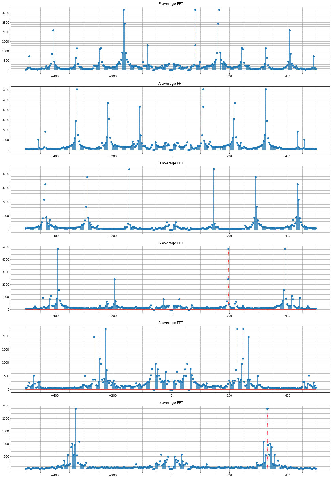
Once I had these average frequency domain signals for each guitar string, I could normalize them and create unit vectors. I could then perform a dot product between any frequency domain signal and my unit vectors, and the result would give me a measure of how similar the two vectors are.
If I have 256 point frequency domain signal, \(\vec{a}\), and a unit vector, \(\vec{b}\), (since \(\lvert\vec{b}\rvert = 1\)), their dot product is given by: $$ \lvert\vec{a}\rvert \lvert\vec{b}\rvert cos(\theta) = \lvert\vec{a}\rvert cos(\theta) $$ where \(\theta\) is the angle between the two vectors. Increasing \(\theta\) decreases the result of the dot product. Therefore the greatest possible value that can result from this dot product is the case where \(\lvert\vec{a}\rvert\) points in the same same direction as \(\lvert\vec{b}\rvert\).
The code below calculates the 6 unit vectors for each guitar string. To decrease dot product computations, I decided that my unit vectors did not need to take into account all of the frequencies in the frequency domain. Given the symmetry of the signals, I could instantly remove half the signal and still keep all of the information. So I only care about positive frequencies. I also did not care about all frequency bins. My interest is only in frequencies around the ideal guitar string frequencies. For example, my guitar tuner would not expect to hear a 50Hz sound. It would expect to hear sounds that are fairly close to the guitar string frequencies. For this reason my unit vectors represented the FFT coefficients for frequency bins at the following frequencies:
print(frequencies_of_interest)[74.2188, 78.125, 82.0312, 85.9375, 89.8437, 101.5625, 105.4687, 109.375, 113.2812, 117.1875, 140.625, 144.5312, 148.4375, 152.3438, 156.25, 160.1562, 164.0625, 167.9687, 171.875, 187.5, 191.4062, 195.3125, 199.2187, 203.125, 210.9375, 214.8437, 218.75, 222.6562, 226.5625, 238.2812, 242.1875, 246.0937, 250.0, 253.9062, 285.1562, 289.0625, 292.9688, 296.875, 300.7812, 320.3125, 324.2187, 328.125, 332.0312, 335.9375, 382.8125, 386.7187, 390.625, 394.5312, 398.4375, 402.3437, 406.25, 410.1562, 414.0625, 417.9687, 433.5937, 437.5, 441.4062, 445.3125, 449.2187]
unit_vecs = dict.fromkeys(strings)
for k in unit_vecs.keys():
    unit_vecs[k] = get_eigen_fft(fft_signals[k], frequencies_of_interest)

fig, a = plt.subplots(6,1)
for i,k in enumerate(unit_vecs.keys()):
    a[i].stem(frequencies_of_interest, unit_vecs[k], use_line_collection=True)
    a[i].grid(which='both')
    a[i].minorticks_on()
    a[i].set_title(k+' unit vector')
plt.show()
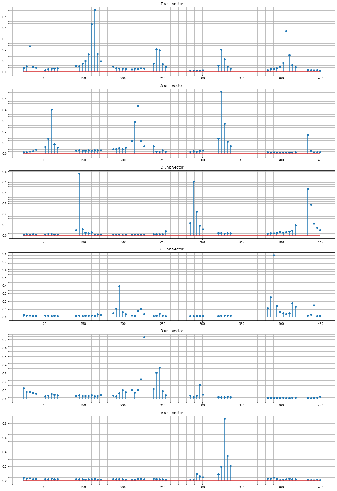
It is interesting to see the profile of each guitar string. We can see that the E string has a prominent second harmonic, and the A string has prominent second and third harmonics. I am curious how much variability there would be if I created unit vectors for different guitars or even different guitar string materials (steel vs nylon).
Let us verify how accurately these unit vectors can predict the guitar string being played. First let’s create a matrix to hold our unit vectors as rows.
proj_matrix = np.matrix(list(unit_vecs.values()))
proj_matrix.shape
(6, 59)
print('Actual \t Predicted')
for st in strings:
    for i in range(4):
        signal = np.array([fft_signals[st][i][f] for f in frequencies_of_interest])
        # project signal onto unit vector matrix. Find string corresponding to largest value
        prediction = strings[ (proj_matrix @ signal).A.argmax() ]
        print(st,'\t', prediction)
Actual   Predicted
E	    E
E    	    E
E    	    E
E    	    E
A    	    A
A    	    A
A    	    A
A    	    A
D    	    D
D    	    D
D    	    D
D    	    D
G    	    G
G    	    G
G    	    G
G    	    G
B    	    B
B    	    B
B    	    B
B    	    B
e    	    e
e    	    e
e    	    e
e    	    e
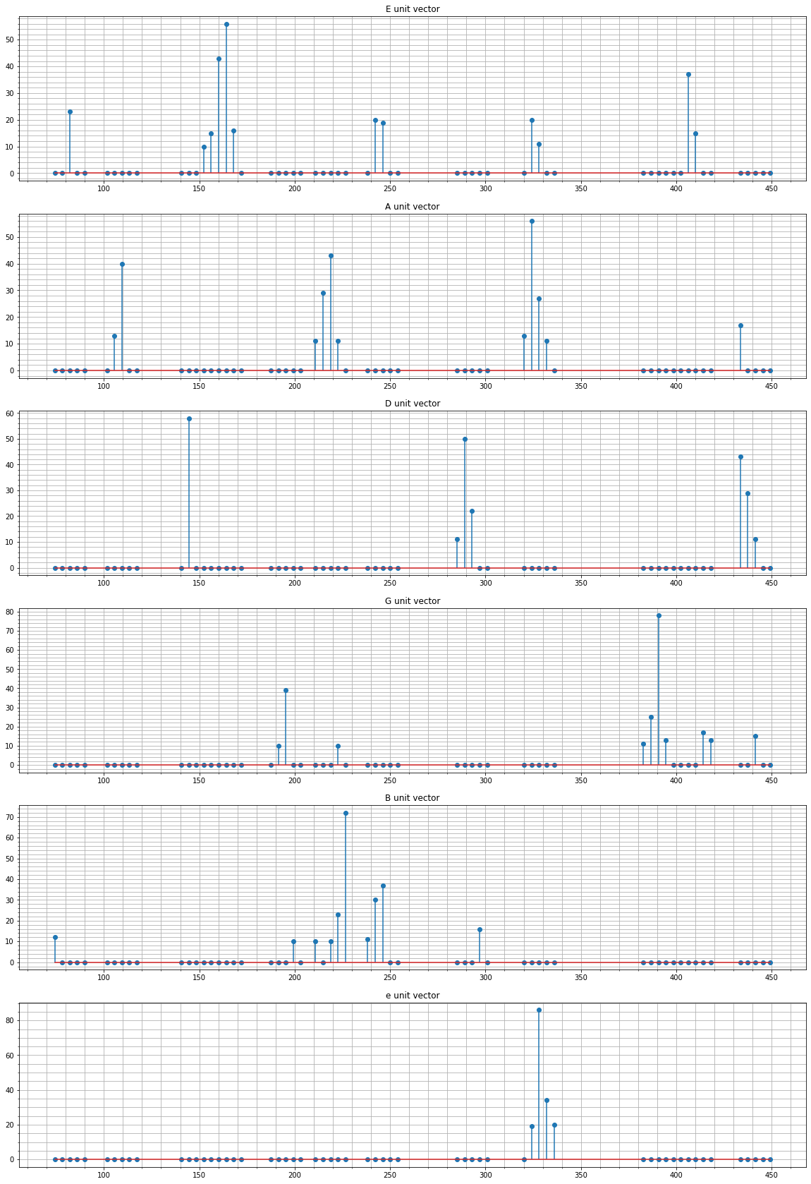
The unit vector approach yields perfect results when tested against the sampled signals. Since this prediction will be running on the STM32, I decided to minimize the number of floating point operations by taking all of the unit vectors and removing any ‘noise’. I removed all components with a value less than 0.1 . Next I multiplied each value by 100 and rounded to the nearest integer. Although the vectors are no longer unit vectors, they should have similar magnitudes, and we can still make reasonable classifications as we have before.
for k in unit_vecs.keys():
    for i, val in enumerate(unit_vecs[k]):
        if val < 0.1: unit_vecs[k][i] = 0
        else: unit_vecs[k][i] = int(unit_vecs[k][i]*100)

for k in unit_vecs.keys():
    print(np.linalg.norm(unit_vecs[k]))
94.71536306217698
95.62949335848225
96.33275663033837
96.96906723280368
93.82430388763883
96.50388593212193
fig, a = plt.subplots(6,1)
for i,k in enumerate(unit_vecs.keys()):
    a[i].stem(frequencies_of_interest, unit_vecs[k], use_line_collection=True)
    a[i].grid(which='both')
    a[i].minorticks_on()
    a[i].set_title(k+' unit vector')
plt.show()
Estimating frequency
After making a prediction about which string is being played, I could then look at the frequency domain signal around the frequency of interest to make an estimate of the fundamental frequency. I did this by taking a weighted average of FFT coefficients around the frequency of interest. The plot below shows a spectrograph of an e string, and in red are the frequency bins used to calculate the weighted average. The e string has an ideal frequency of 330 Hz, and the weighted average predicts the signal to have a fundamental frequency of 329.57 Hz.
freq = list(fft_signals[‘e’][0].keys())
mag = list(fft_signals[‘e’][0].values())
plt.stem(freq[:128], mag[:128], use_line_collection=True)

i = freq.index(328.125)
plt.stem(freq[i-1:i+3], mag[i-1:i+3], ‘r’, use_line_collection=True)

plt.title(‘e FFT’)
plt.grid()

plt.gcf().set_size_inches(20,6)
plt.show()

print('%.2f Hz'%weighted_average(freq[i-1:i+3], mag[i-1:i+3] ))
329.57 Hz
Conclusion
The analysis shown in this notebook is the algorithm I used to take a 256 point frequency domain signal of a recorded guitar string and predict the fundamental frequency. This is the algorithm that is running on the STM32, with the unit vectors obtained by this analysis.
Not displayed are the other approaches I took that did not work well. I first tried a naive approach where I predicted the fundamental frequency to be the greatest component in the frequency domain signal. This failed due to harmonics. The other approach was to use autocorrelation. This also failed since it was difficult to distinguish between the A and e string, as well as the E and B string. This is because their frequencies are multiples of each other ( A -> 110 Hz, e->330 Hz ) and I had no way of distinguishing between these strings effectively.
Implementation
Once I had the unit vectors and the algorithm working in Python, I then had to implement that on the STM32.
Block Diagram
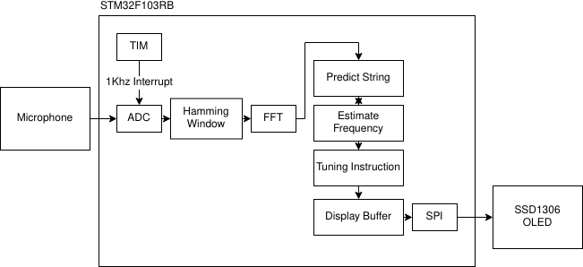
In summary the STM32 uses several peripherals. A timer is used to generate interrupts at 1KHz. The interrupt service routine reads converted data from the ADC peripheral and fills a buffer that can hold 256 float values. SPI is used to drive the OLED display.
In main(), we setup all peripherals, initialize the OLED display and then enter a while loop. The while loop constantly checks if the buffer is filled with values. If the buffer is full, we disable the timer interrupt, perform an FFT, predict the guitar string being played, estimate the fundamental frequency, fill the OLED display buffer with proper tuning instructions, write to the OLED and re-enable the timer interrupt.
For full code see github
while(1)
    {
    Delay(10);
    if(buffer_count == ADC_BUFF_SIZE) // Check if adc_buffer is filled with values
    {
        TIM_ITConfig(TIM2, TIM_IT_CC1, DISABLE); // Disable TIM2 interrupt

    fft(fft_samples, ADC_BUFF_SIZE, temp);
    get_magnitudes(mag, fft_samples, ADC_BUFF_SIZE);
    filter_frequencies(mag, freq, 0.0, 4.0, ADC_BUFF_SIZE);
    filter_frequencies(mag, freq, 60.0, 5.0, ADC_BUFF_SIZE);

    // Dot product of unit_vecs with signal fft
    int i;
    float dp[6] = {0};
    for(i=0; i<UNIT_VEC_LENGTH; i++)
    {
	float f = eigen_frequencies[i];
	int index = freq_to_index(f, 1000, ADC_BUFF_SIZE);
	dp[E] += E_fft_unit_vec[i] * mag[index];
	dp[A] += A_fft_unit_vec[i] * mag[index];
	dp[D] += D_fft_unit_vec[i] * mag[index];
	dp[G] += G_fft_unit_vec[i] * mag[index];
	dp[B] += B_fft_unit_vec[i] * mag[index];
	dp[e] += e_fft_unit_vec[i] * mag[index];
    }

    // find max string
    float max_val = 0.0;
    int max_index;
    for(i=0; i<6; i++)
    {
	if(dp[i] > max_val)
	{
	    max_val = dp[i];
	    max_index = i;
	}
    }

    if(UART_DEBUG)
    {
	char buffer[20];
	/*
	// Send string prediction over uart
	switch(max_index)
	{
	    case E: sprintf(buffer, "String: %s \n\r", "E");
	    break;
	    case A: sprintf(buffer, "String: %s \n\r", "A");
	    break;
	    case D: sprintf(buffer, "String: %s \n\r", "D");
	    break;
	    case G: sprintf(buffer, "String: %s \n\r", "G");
	    break;
	    case B: sprintf(buffer, "String: %s \n\r", "B");
	    break;
	    case e: sprintf(buffer, "String: %s \n\r", "e");
	    break;
	}
	uart_puts(buffer, USART1);
	*/

	float estimated_freq = estimate_frequency(mag, freq, max_index);
	if(max_index==E) estimated_freq /= 2;
	if(max_index==A) estimated_freq /= 3;
	sprintf(buffer, "%.4f\n\r", estimated_freq);
	uart_puts(buffer, USART1);
    }

    last4[temp_index] = estimate_frequency(mag, freq, max_index);

    // float estimated_freq = estimate_frequency(mag, freq, max_index);
    float estimated_freq = last4_average(last4, temp_index);
    temp_index = (temp_index+1)%4;

    float difference;
    switch(max_index)
    {
        // case E: difference =  estimated_freq -  E_freq;
        case E: difference =  estimated_freq/2 -  E_freq;
            break;
        case A: difference =  estimated_freq/3 -  A_freq;
            break;
        case D: difference =  estimated_freq -  d_freq;
            break;
        case G: difference =  estimated_freq -  G_freq;
            break;
        case B: difference =  estimated_freq -  B_freq;
            break;
        case e: difference =  estimated_freq -  e_freq;
            break;
    }

    uint8_t display_buff[NUM_BYTES];
    tuning_instruction(difference, display_buff, max_index);

    ssd1306_display_buffer(display_buff);
    Delay(20);

    buffer_count = 0;
    TIM_ITConfig(TIM2, TIM_IT_CC1, ENABLE);
    // break;
}
}